Decreasing Viola-Jones False positives: A new approach
Viola Jones
Viola Jones is perhaps one of the oldest object detection algorithms, the paper was released in 2001 by Paul Viola & Michael Jones. The idea was to use Haar-like features within a cascaded ensemble approach to detect objects.
Haar-like features
A rectangular feature in which light pixels (within the feature) corresponds to light pixels in the image and vice versa. These features can be thought of as rectangular patterns within an image. For example a haar feature for a nose is a rectangular feature where 2 parts of it are dark and the middle part is light as seen in the following image. (Credits to: Real Python)
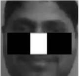
Nose feature
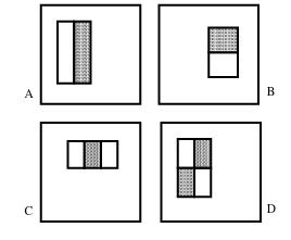
Rectangular Features
Ensemble
Unlike other object detection algorithms, the Viola-Jones algorithm uses an ensemble approach to output an accurate classification. This means that instead of using a single strong classifier, Viola-Jones uses multiple weak classifiers where each contributes to the final classification. Each weak classifier works with a single Haar-like feature.
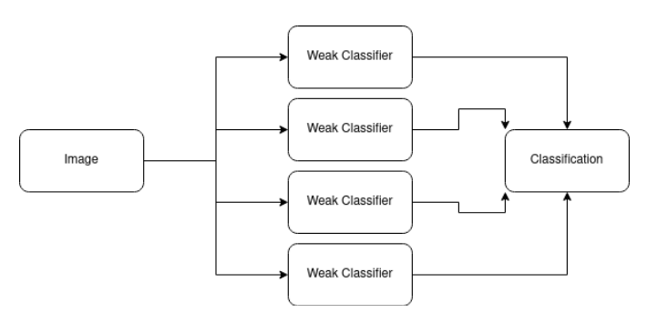
Ensemble Approach for classification
Cascade
For a realtime and extremely fast object detection we need to remove false inputs from consideration as easily as possible. This is where the Cascade approach comes in. We train multiple Viola-Jones models with increasing complexity (i.e. number of features/classifier is increasing). At each stage, whenever a model outputs that the input is false, the cascade short circuits and outputs a false classification.
This post is not intended to be a reference for viola-jones which is why I’m not going to further discuss how it works. To learn more about the algorithm check out this repo and also check his articles on medium, the above is kind of a summary for his articles.
Decreasing any false positives.
There’s a neat way to decrease the rate of false positives in most if not all algorithms which is to limit or narrow down the search space of the algorithm. This doesn’t just provide a better FPR but it also leads to better performance.
The pipeline that we used for better FPR rate for Viola-Jones face detection is as follows:
- Skin Color segmentation (Get skin pixels only)
- Morphological Erosion (Remove dots & small imperfections)
- Gaussian Filter (Smooth down the image and remove holes)
- Thresholding with a low threshold (remove holes)
- Mask original image with the output of the thresholding stage.
- Find contours
- Resize each contour and send it to viola-jones
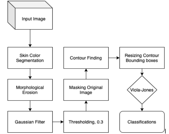
Graphical representation of the new pipeline.
Skin Color Segmentation
There’re multiple ways to segment an image based on skin color, the one I used is simple but yet effective. It is based on the paper:
R. F. Rahmat, T. Chairunnisa, D. Gunawan and O. S. Sitompul, “Skin color segmentation using multi-color space threshold,” 2016 3rd International Conference on Computer and Information Sciences (ICCOINS), 2016, pp. 391-396, doi: 10.1109/ICCOINS.2016.7783247.
We start by applying skin color segmentation on the input image using two sets of conditions that either of them must be true. Which are as follows:
- Condition Set (1):
- Normalized red channel divided by the normalized green channel values must be less than 1.185
- Hue channel value must not belong to the interval [0, 25]
- Condition Set (2):
- Hue channel value must not belong to the interval [335, 360]
- Saturation channel value must not belong to the interval [0.2, 0.6]
- Cb channel value must not belong to the interval (77, 127)
- Cr channel value must not belong to the interval (133, 173)
Which can be implemented in Python as follows:
def get_normalized_rgb(img):
  normalizedImg = np.zeros(img.shape)
  normalizedImg = cv2.normalize(np.copy(img),  normalizedImg, 0, 255, cv2.NORM_MINMAX)
  return normalizedImg

def get_hsv(img):
  clone = np.array(np.copy(img), dtype=np.single)
  hsv = cv2.cvtColor(clone, cv2.COLOR_RGB2HSV)
  return hsv

def get_ycbcr(img):
  clone = np.array(img, dtype=np.single)
  ycbcr = cv2.cvtColor(clone, cv2.COLOR_RGB2YCrCb)
  return ycbcr

def segment_skin(image):
  ycbcr = get_ycbcr(image)
  hsv = get_hsv(image)
  normal = get_normalized_rgb(image)

  divided_normal = normal[:,:,0] / normal[:, :, 1]
  divided_normal = divided_normal > 1.185
  clone = np.array(np.copy(image), dtype=np.uint8)

  mask_hsv_lower_h = cv2.inRange(hsv, (0, 0, 0), (25, 255, 255))
  mask_hsv = cv2.inRange(hsv, (335, 0.2, 0), (360, 0.6, 255))
  mask_ycbcr = cv2.inRange(ycbcr, (0, 77, 133), (255, 127, 173))

  rgb_condition = np.logical_and(divided_normal, np.array(mask_hsv_lower_h).astype(bool))

  c1,r1 = np.where(mask_hsv == 0)
  c2,r2 = np.where(mask_ycbcr == 0)
  ones = np.ones((clone.shape[0], clone.shape[1]), dtype=bool)

  ones[c1,r1] = False
  ones[c2,r2] = False

  either = np.logical_or(ones, rgb_condition)

  c,r = np.where(either == False)

  clone[c,r] = [0, 0, 0]

  return clone
The above function segment_skin() takes a NumPy image matrix and segments it based on the above conditions.
The rest of the pipeline is self-explanatory, so we’ll just head to the full code:
Implementation
def get_binary_mask(img):
  black_pixels_mask = np.all(img == [0, 0, 0], axis=-1)
  clone = np.ones((img.shape[0], img.shape[1]), 'uint8')
  clone[black_pixels_mask] = 0
  return clone

def apply_gaussian_binary(img, sigma):
  blurred = skimage.filters.gaussian(img, sigma)
  _max = blurred.max()
  return (blurred * (1 / _max))

def threshold(img, thresh):
  clone = np.array(np.copy(img))
  black_pixels_mask = np.where(clone <= thresh)
  clone[black_pixels_mask] = 0
  return clone

def apply_binary_mask(img, mask):
  mask_data = mask.get_data()
  clone = np.array(np.copy(img))
  black_pixels_mask = np.where(mask == 0)
  clone[black_pixels_mask] = [0,0,0]
  return clone

def crop(img, xmin, xmax, ymin, ymax):
  cropped = img[ymin:ymax+1, xmin:xmax+1]
  return cropped


img = cv2.imread("/path/to/image") # Load NumPy array
img = cv2.cvtColor(img, cv2.COLOR_BGR2RGB) # Convert OpenCV's BGR to RGB

segmented = segment_skin(img)
binary_mask = get_binary_mask(segmented)
eroded = cv2.erode(
  binary_mask,
  [
    [1,1,1],
    [1,1,1],
    [1,1,1],
  ],
  iterations = 1
)

smoothed = apply_gaussian_binary(eroded, 3)

thresholded = threshold(smoothed, 0.3)

masked = apply_binary_mask(img, thresholded)

contours, _ = cv2.findContours(masked, cv2.RETR_TREE, 1)

bounding_boxes = []

for contour in contours:
  x,y,w,h = cv2.boundingRect(c)
  bounding_boxes.append({
    "image": crop(img, x, y, x+w, y+h),
    "x": x,
    "y": y,
    "w": w,
    "h": h
  })

faces = [bounding_box for bounding_box in bounding_boxes if model.classify(resize(bounding_box["image"]))] # Resize according to your viola-jones model

## Show faces
Results
The following are some of the results that the above pipeline achieved:
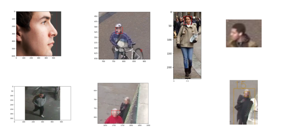
Sample Results of the proposed pipeline
Future work
To improve the current pipeline there are multiple options that come to my mind which are:
- Use Fuzzy/Soft Thresholding for skin color segmentation to account for different illumination
- Adjust AdaBoost formula for the weak classifier to provide better FPR
At the end, the current approach does decrease the amount false positives and when a low threshold is used for the Viola-Jones model, we can locate faces even VGG cannot. However it’s still not accurate enough to compete with modern Deep learning approaches but still it provides great performance over the other CNN approaches.